A deep dive into geographic image classification using Google Street View and Convolutional Neural Networks
Can a Neural Network Tell You Where in the World You Are?
Ibuilt several Convolutional Neural Networks, in Python using the PyTorch library, to classify Google Street View images by country. I compared custom-built architectures against transfer learning approaches, experimenting with different loss functions, and learning a lot about what makes geographic image classification so surprisingly hard.
Cover image source: The Scientist
Introduction
I love to travel. Over the years I’ve been lucky enough to visit Canada, Czechia, Estonia, Finland, Germany, Italy, Japan, Latvia, Lithuania, Mexico, Peru, Slovakia, Spain, Sweden, and the United States. At some point, naturally, I started wondering: could a machine learning model look at a photo and figure out which of those countries it came from?
That question turned into a full project for my machine learning course, and the results were genuinely interesting, both in terms of what the model got right and where it struggled. In this post I’ll walk you through the data, the models I built, the loss functions I experimented with, and what I found.
The Data
The images all come from Google Maps Street View, pulled from a Kaggle dataset that originally contained roughly 50,000 images spanning 124 countries. I filtered it down to my 15 countries and immediately ran into a classic machine learning headache: class imbalance.
The US alone had over 12,000 images. Japan came in second with around 4,000. Meanwhile Latvia, Slovakia, and Estonia each had barely 100 images. If you throw that at a model, it’ll quickly learn to guess “United States” for almost everything and still look decent on paper.
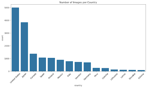
To deal with this, I randomly sampled 5,000 US images, bringing my total dataset to roughly 12,000 images across 15 countries. Each image was resized to 224×224 pixels, and I performed an 80/20 training/validation split using stratified sampling — meaning each country was represented proportionally in both sets.
What Is a Convolutional Neural Network?
Before jumping into the results, it’s important to know what a Convolutional Neural Network is.
A Convolutional Neural Network (CNN) is a type of neural network designed specifically for image data. Rather than treating every pixel as an independent input (which would be extremely computationally intensive for a 224×224 image), CNNs use convolutional layers that scan small patches of the image with learned filters. Early layers tend to detect simple things like edges, colors, and gradients. Deeper layers combine those into more complex patterns such as textures, shapes, and eventually objects or scenes.
CNNs have become the backbone of modern computer vision. They power everything from facial recognition to self-driving cars to, as it turns out, guessing which country a street looks like it belongs to.
What Is Transfer Learning?
One of the most powerful ideas in modern deep learning, however, is that you don’t always have to start from scratch.
Imagine training a model on millions of photos to recognize everyday objects — cars, trees, buildings, skies, roads. In doing so, the model’s early layers learn incredibly general and reusable visual features: how to detect edges, how to recognize textures, how sky looks different from asphalt. That general knowledge transfers.
Transfer learning means taking a model that was already trained on a large dataset and repurposing it for a new task. Instead of randomly initializing all of the model’s weights and hoping the model figures out what an edge is from scratch, you start with weights that already encode rich visual understanding, and then train the whole thing further on your specific problem.
For this project I used two pre-trained ResNet50 architectures, which is a well-known 50-layer CNN. One was originally trained on ImageNet (a massive dataset of everyday objects) and the other on Places365 (a dataset specifically designed around scenes and places, exactly the kind of thing that might help with geography). Both were fully trainable, meaning I didn’t freeze any layers; the entire network was allowed to continue learning from my Street View data.
Loss Functions: Teaching the Model What “Wrong” Means
A loss function is how you tell a neural network how badly it’s doing. During training, the model makes predictions, you compute the loss, and then you backpropagate that signal through the network to update the weights. Different loss functions encode different ideas about what kinds of mistakes matter.
I tested three for the from-scratch models:
Cross-Entropy Loss (Baseline)
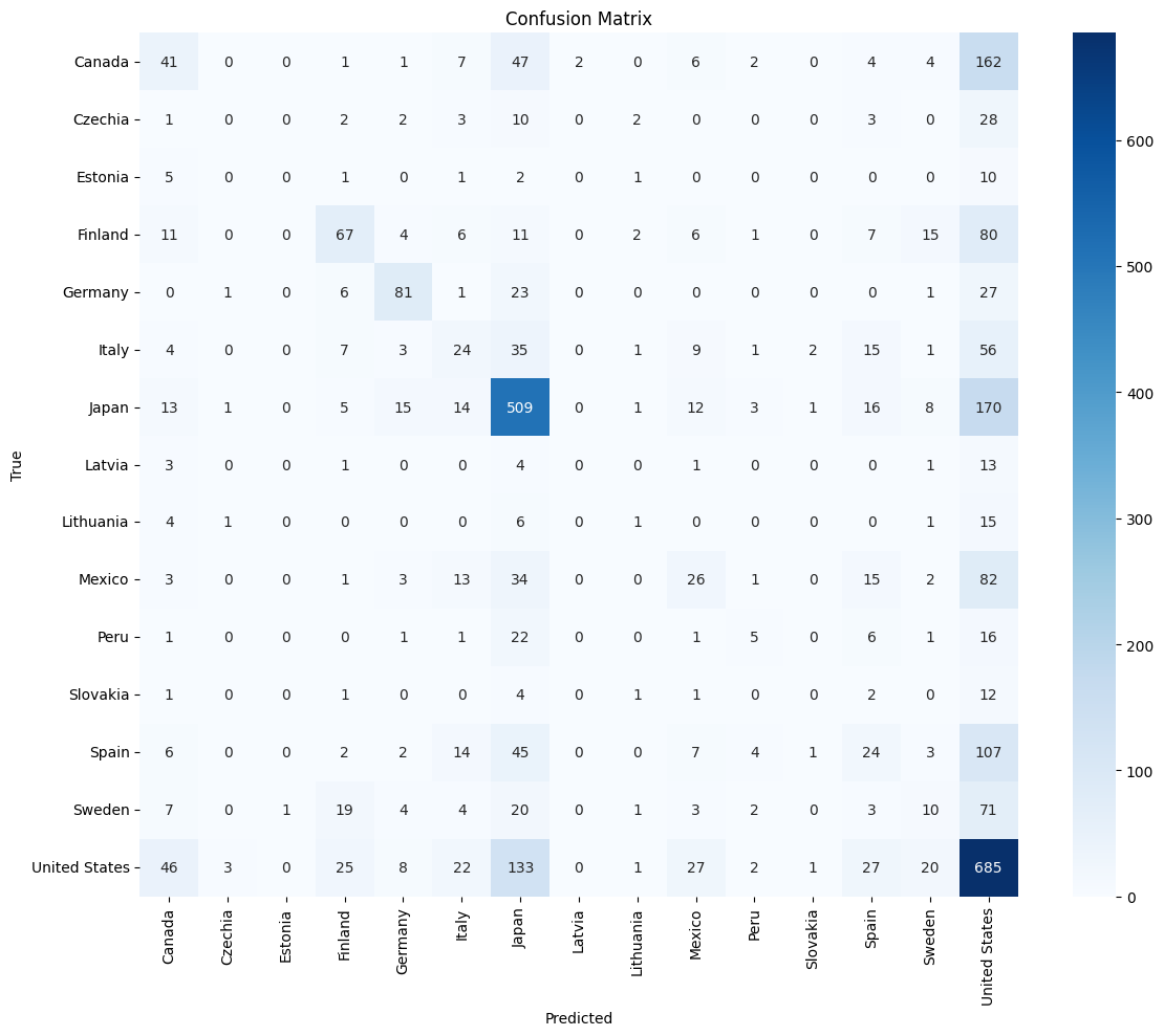
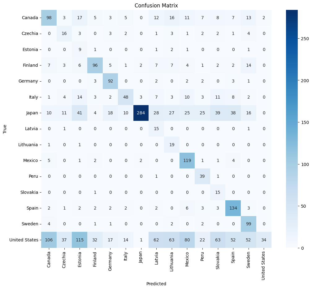
The standard choice for classification. It penalizes the model in proportion to how confident it was in a wrong answer. Clean and simple, but it has a problem with imbalanced classes: the model can minimize loss by just learning to confidently predict the majority class (US and Japan, in my case). Looking at the confusion matrix for this model, that’s pretty much exactly what happened.
Weighted Cross-Entropy
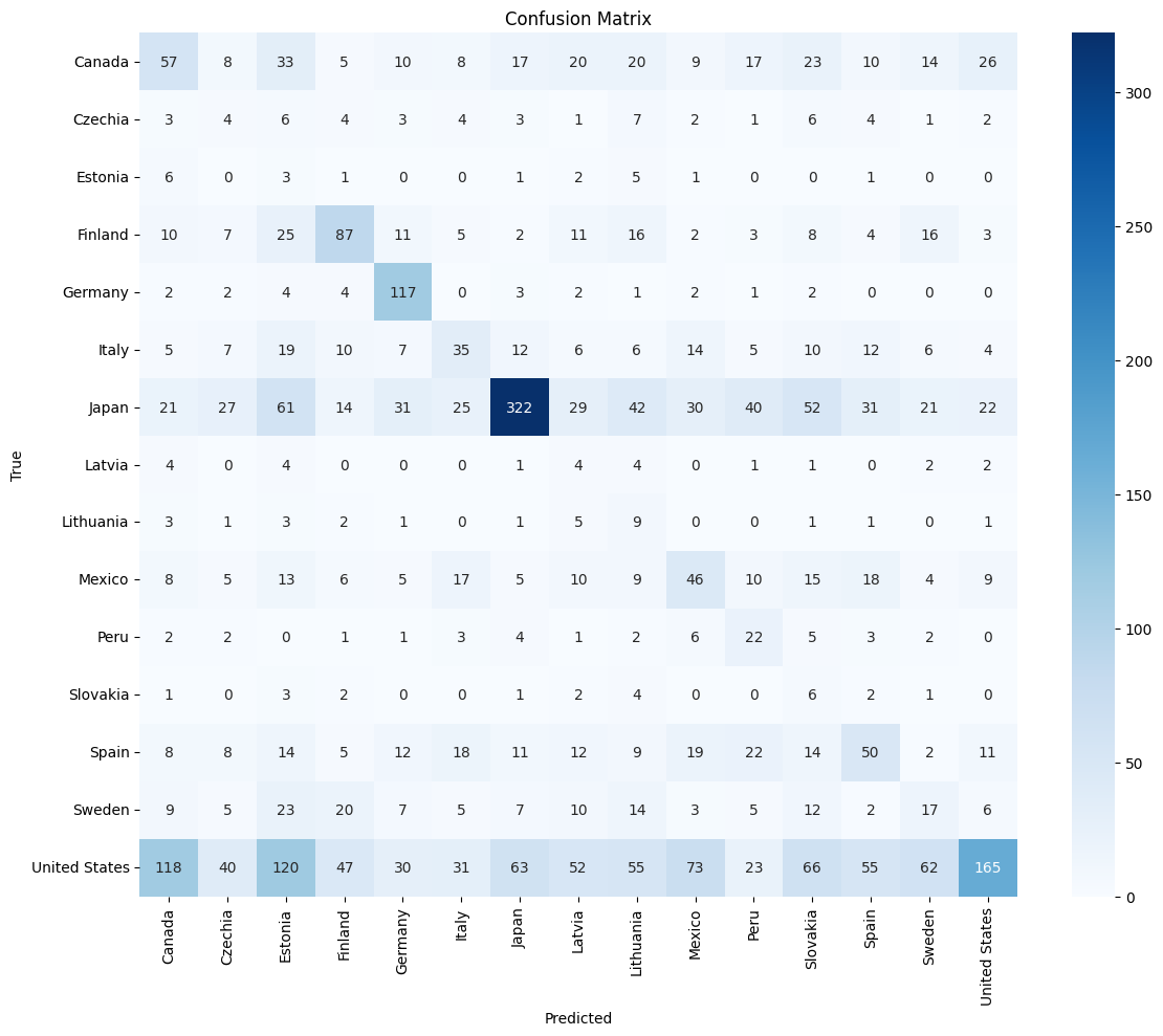
A straightforward fix for class imbalance: assign larger penalties for getting minority classes wrong. In theory this should push the model to pay more attention to Latvia and Estonia. In practice, this model ran for 48 epochs (compared to 6 for the others) and achieved a validation accuracy of only 28.68%, which is worse than the baseline, and had nowhere near as good of a top-5 accuracy either. The training became unstable and the model seemed to overcorrect, but at least the model wasn’t guessing the US and Japan essentially every time anymore.
Focal Loss
This is the interesting one. Focal loss is a modified version of cross-entropy that dynamically downweights easy examples. The key insight: if the model is already very confident about a prediction, it probably doesn’t need to spend much more time on that example. But if it’s uncertain (if a small, visually ambiguous class keeps tripping it up) the loss stays large and the model keeps focusing there.
Mathematically, focal loss multiplies the standard cross-entropy term by a factor of (1 - p_t)^γ, where p_t is the predicted probability for the correct class and γ is a tunable hyperparameter. When p_t is high (easy examples), this factor is close to zero and the loss shrinks. When p_t is low (hard examples), the factor is close to 1 and the loss behaves like standard cross-entropy.
Here’s how the focal loss is implemented in PyTorch:
class FocalLoss(nn.Module):
    def __init__(self, gamma=2.0, reduction='mean'):
        super(FocalLoss, self).__init__()
        self.gamma = gamma
        self.reduction = reduction

    def forward(self, inputs, targets):
        ce_loss = F.cross_entropy(inputs, targets, reduction='none')
        pt = torch.exp(-ce_loss)
        focal_loss = ((1 - pt) ** self.gamma) * ce_loss
        if self.reduction == 'mean':
            return focal_loss.mean()
        return focal_loss.sum()
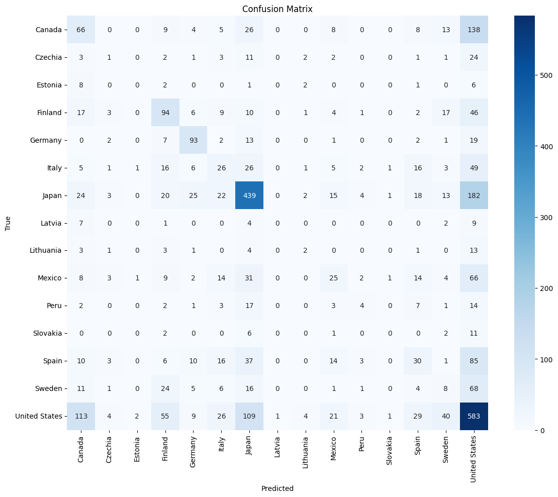
The result: the focal loss model converged in just 6 epochs and outperformed both other custom architectures.
The From-Scratch Architecture
The custom CNNs I built follow a standard pattern: alternating convolutional layers, batch normalization, ReLU activation, and max pooling to progressively extract features and reduce spatial dimensions, followed by fully connected layers at the end to produce class predictions. Here’s a simplified look at the architecture:
class CustomCNN(nn.Module):
    def __init__(self, num_classes=15):
        super(CustomCNN, self).__init__()
        self.features = nn.Sequential(
            nn.Conv2d(3, 32, kernel_size=3, padding=1),
            nn.BatchNorm2d(32),
            nn.ReLU(),
            nn.MaxPool2d(2, 2),

            nn.Conv2d(32, 64, kernel_size=3, padding=1),
            nn.BatchNorm2d(64),
            nn.ReLU(),
            nn.MaxPool2d(2, 2),

            nn.Conv2d(64, 128, kernel_size=3, padding=1),
            nn.BatchNorm2d(128),
            nn.ReLU(),
            nn.MaxPool2d(2, 2),
        )
        self.classifier = nn.Sequential(
            nn.Dropout(0.2),
            nn.Linear(128 * 28 * 28, 512),
            nn.ReLU(),
            nn.Dropout(0.2),
            nn.Linear(512, num_classes)
        )
All custom models shared the same training setup:
- 20% dropout to reduce overfitting
- Weight decay of 0.0001 as regularization
- Data augmentation (random flips, color jitter, etc.) during training
- An adaptive learning rate scheduler
- Early stopping with a patience of 5 epochs
I also tried a fine-tuned variant where I first trained rigorously on the majority classes, then fine-tuned on the smaller ones. This ran for a combined 50 epochs (30 on majority, 20 for fine-tuning) and ended up being the most computationally expensive approach.
The Pre-Trained Models
For the transfer learning models, loading a ResNet50 pre-trained on Places365 and making it fully trainable looks like this:
import torchvision.models as models

model = models.resnet50(pretrained=False)
model.load_state_dict(torch.load('resnet50_places365.pth'))

# Replace final layer for 15-class output
model.fc = nn.Linear(model.fc.in_features, 15)

# All layers trainable — no freezing
for param in model.parameters():
    param.requires_grad = True
Both the ImageNet and Places365 variants followed this same pattern, with only the pre-trained weights differing between them.
Results
Here’s how all six models compared:
| Model | Loss Function | Epochs | Val Accuracy | Macro F1 | Top-5 Val Accuracy |
|---|---|---|---|---|---|
| Custom Baseline | Cross-Entropy | 6 | 44.76% | 0.2086 | 84.75% |
| Custom Weighted | Weighted CE | 48 | 28.68% | 0.2214 | 53.75% |
| Custom Focal | Focal | 6 | 41.66% | 0.2111 | 85.05% |
| Custom Fine-Tuned | Focal (2-stage) | 30+20 | 45.26% | 0.4277 | 59.68% |
| ResNet (ImageNet) | Focal | 14 | 35.82% | 0.2162 | 85.60% |
| ResNet (Places365) | Focal | 6 | 34.97% | 0.2119 | 84.99% |
A few things jump out here.
Top-5 accuracy is where the real story is. Rather than asking whether the model picked the exact right country, top-5 accuracy asks whether the correct country appeared somewhere in the model’s top 5 guesses. The best custom model (focal loss) hit 85.05%, and the Places365 pre-trained model was essentially tied at 84.99%. For a 15-class problem with genuinely ambiguous images, that’s pretty good behavior.
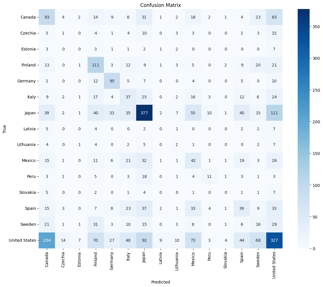
The baseline model looks great until you look at the confusion matrix. Cross-entropy on an imbalanced dataset leads to exactly the pathology you’d expect: the model learns to almost always predict US or Japan, which are the two largest classes. High accuracy on those, near-zero on everything else, almost 85% top-5 accuracy. However, the macro F1 score of 0.21 gives it away.
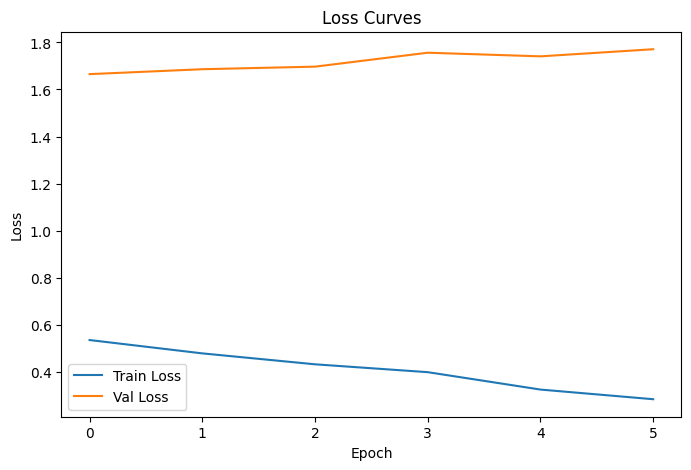
The focal loss model overfits. Training accuracy of 96.22% vs. validation accuracy of 41.66% is a wide gap. The pre-trained models are much more balanced. The Places365 ResNet had 79.54% training accuracy vs. 34.97% validation, which is still overfitting but noticeably less severe.
The pre-trained Places365 model is the overall winner. Not because its validation accuracy was highest (the fine-tuned model edges it out there), but because it generalizes better, converged in just 6 epochs, and was more calibrated in its uncertainty.
Uncertainty and Model Calibration
Beyond raw accuracy, I also looked at how confident the model was and whether that confidence was warranted.
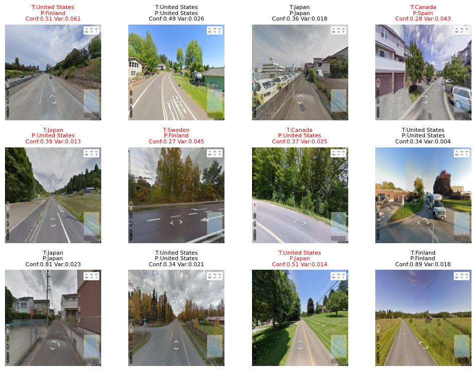
Prediction confidence and variance were computed using MC-Dropout: running the model multiple times with dropout active during inference and averaging the results. This gives both a mean prediction and a variance that reflects how uncertain the model is.
def mc_dropout_predict(model, image, n_passes=50):
    model.train()  # Keep dropout active
    predictions = []
    with torch.no_grad():
        for _ in range(n_passes):
            output = torch.softmax(model(image), dim=1)
            predictions.append(output.cpu().numpy())
    predictions = np.array(predictions)
    mean_pred = predictions.mean(axis=0)
    variance = predictions.var(axis=0)
    return mean_pred, variance
What I found was actually interesting: when the model correctly predicted a large class like the US (54% confidence) or Japan (66%), its confidence was moderate. When it misclassified a medium-sized class like Mexico or Canada, confidence was quite low (around 21–29%). But when it correctly nailed a small class like Finland, confidence jumped to 81%. That’s focal loss doing exactly what it was designed to do — pushing the model to really learn the minority classes rather than treating them as afterthoughts.
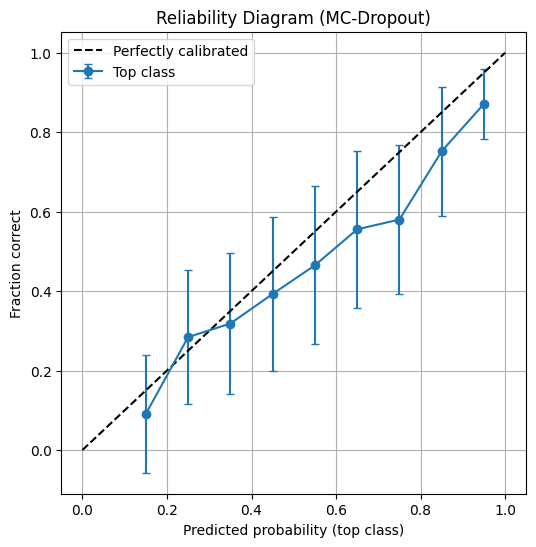
The reliability diagram plots predicted probability against actual fraction correct. A perfectly calibrated model would fall exactly on the diagonal. The Places365 model tracks reasonably well in the middle ranges but overestimates confidence at high predicted probabilities, which is a common pattern for deep neural networks.
Limitations and What I’d Do Differently
Honestly, there is still a lot of room to improve here.
The dataset is small for deep learning. 12,000 images sounds like a lot, but ResNet50 has 25 million parameters. It was always going to struggle to generalize fully.
Street View images are inherently noisy. Most images are some variation of “road with trees on the side.” There just aren’t that many distinguishing features, and there’s enormous visual diversity even within a single country. A Swedish highway looks a lot like a Finnish highway.
Some images contain obvious giveaways. Country flags, road signs in specific languages, license plates. It would be genuinely interesting to split the dataset into “images with text/flags” and “images with just scenery” to see if the model is learning real geographic features or just reading signs.
Computational constraints. I was definitely limited in how much I could experiment with architecture size and hyperparameters due to computation time and intensity.
Future directions I’d be curious about: grouping countries into continents to reduce the classification difficulty while using the full original dataset, deeper analysis of which country pairs get confused most often and why, and more aggressive data augmentation or image cleaning to strip out obvious country identifiers.
Final Takeaway
Geographic image classification is a hard problem. Street View images from different countries can look remarkably similar, and visual cues are subtle. But even with a modest dataset and relatively simple architectures, focal loss helped push a custom CNN to 85% top-5 validation accuracy, and a ResNet pre-trained on scene-level images matched that essentially exactly while generalizing far better.
The main lesson I took away isn’t really about geography. It’s about loss functions. The choice of how you define “wrong” shapes everything about how your model learns. Cross-entropy on an imbalanced dataset produces a model that learns to be confidently lazy. Focal loss forces it to keep working on the hard cases, and the difference shows up clearly in the results.
The full code is available on my GitHub. There are three total notebooks: one for EDA, one for the from-scratch architectures and one for the pre-trained models.